Experimenting with Maximal Coding Rate Reduction
12 Jun 2022 - Dean Goldman
Introduction
I do a lot of work developing deep learning models for multiclass classification. An important part of this process is to engineer an objective function that optimizes for representations that are similar for samples within-class, and dissimilar for samples between-class. The idea is that if we’re interested in performing multiclass classification for some unseen sample, our model should project that sample onto a coordinate in a hidden space such that that coordinate is closest to other samples’ coordinates of the same class. There are plenty of different ways to train a model toward this objective, in this post I investigate an approach that was new to me: the Principle of Maximal Coding Rate Reduction, or MCR\(^2\) (Ma, et al.). I describe a bit about what this loss function theoretically achieves, and I compare it to some baseline loss functions that can be used for contrastive learning- like taking the within/between class L2-norm, and Fisher’s Linear Discriminant. The goal here is not necessarily to make a case for any one approach, but to explore the behavior of different loss functions, understand some of the theory behind them, and iterate over a few experiments.
Maximal Coding Rate Reduction
The fundamental idea behind MCR\(^2\) is that there is a theoretical minimum number of bits required to encode a set of vectors \(W\), with a given amount of distortion \(\epsilon\), into a region \(\mathbb{R}^{n}\). This is basically to say that a space \(\hat{W}\) can give a unique encoding to every vector \(w_{i} \in W\) down to a margin of error (it can’t encode between the error bounds), and there is a minimum number of bits needed to do so. The authors of the MCR\(^2\) use a sphere-packing explanation to illustrate their point.
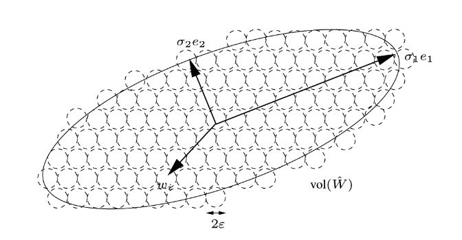
A subtle detail to note is that \(\text{Vol}(\hat{W})\) is said to be proportional to the determinant of the covariance matrix of \(W\). The useful aspect of measuring the covariance matrix has to do with the expectation that samples from different clusters will be uncorrelated, so their within-class covariance matrices will generally look different from the between class covariance matrices. To dive into a little more detail, the covariance matrix looks like:
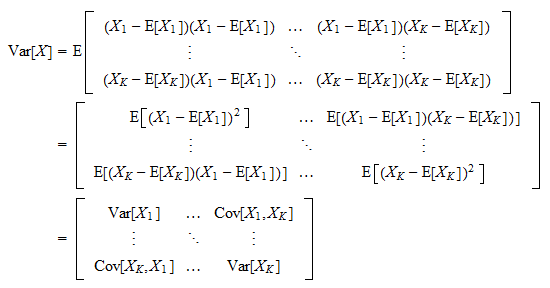
If we partition a space \(W\) to include only those samples of a particular class, we would be looking at how each dimension covaries with another within this class partition. As we addd the class partitions back in, we may expect to see more deviation from the mean, as some dimensions contain clusters of samples in one class far from samples in other classes. This expected increase in covariance is fundamental to the objective function, which will be looked into more.
Filling the space \(\text{Vol}(\hat{W})\) with \(\epsilon\)-spheres with volume \(\text{vol}(z)\) can be expressed algebraically as:
So the expected number of bits to label a sphere coinciding with any vector \(w_{i}\) in \(W\) can be expressed as a function \(R(W)\): (This is equation 11 in [2])
\[\begin{aligned} R(W) &= \text{log}_{2} (\text{# of spheres})\\ &= \text{log}_{2}(\text{Vol}(\hat{W}) / \text{vol}(z)) = \frac{1}{2} \text{log}_{2} \text{det}(I + \frac{n}{m\epsilon^{2}}WW^{T}) \end{aligned} \tag{2}\]Extending this to the number of samples (\(m\)), and number of dimensions (\(n\)) produces equation 13 in the author’s paper, which defines the number of bits needed to encode all \(m\) vectors in \(W \subset \mathbb{R}^{n}\), subject to squared error \(\epsilon^{2}\) [2]:
\[L(W) = (m+n)R(W) = \frac{(m+n)}{2} \text{log}_{2} \text{det}(I + \frac{n}{m\epsilon^{2}}WW^{T}) \tag{3}\]I’ll make an attempt to briefly explain this formula as best as I can. The log-determinant of a Gaussian distribution’s covariance matrix is an expression of the entropy of that Gaussian distribution. To break it all down, the determinant computes the volume of an n-dimensional parallelepiped, in this case the covariance matrix, in units of \(\epsilon\)-spheres [5]. If we’re dealing with a high volume covariance, it is to say that there’s a high variance in the distribution, and because of that there is more uncertainty about what value a sample from that distribution may take (more entropy). Likewise, if it is low there is less variance in the data, there’s less uncertainty, and less entropy. The \(\frac{(m+n)}{2} \text{log}_{2}\) element comes from the Rate-distortion theorem [3]. The proof of the Rate-distortion theorem relies on the measurement of mutual information, or the average amount of information that is communicated in one variable about another [6]. In the proof, the mutual information \(I(X; \hat{X})\) represents the mutual information betweeen an encoding \(\hat{X}\), and it’s source \(X\). This ends up being the difference between two terms (equations 4-6 are all copied or derived from [3]):
\[I(X; \hat{X}) = h(X) - h(X \vert \hat{X}) \tag{4}\]The last term is the conditional entropy: the entropy of \(X\) given that \(\hat{X}\) is known. Or in other words, the uncertainty about \(X\) given that we have its encoding \(\hat{X}\). Since \(\hat{X}\) is given, we can rewrite this term as the entropy of the encoding error:
\[h(X \vert \hat{X}) = h(X - \hat{X} \vert \hat{X}) \tag{5}\]Since conditioning reduces entropy, i.e. we can expect to be less surprised about \(X\) or \(X-\hat{X}\) if we know \(\hat{X}\), we can say that this will always be the case:
\[\begin{aligned} h(X) - h(X-\hat{X} \vert \hat{X}) &\ge h(X) - h(X-\hat{X})\\ I(X; \hat{X}) &\ge h(X) - h(X-\hat{X}) \end{aligned} \tag{6}\]Since the entropy of a Gaussian is known to be: \(\frac{1}{2}\text{log}(2\pi e )\sigma^{2}\), we can substitute this into the lower bound (this is equation 10.31 in [3]):
\[I(X; \hat{X}) = \frac{1}{2}\text{log}(2\pi e )\sigma^{2} - \frac{1}{2}\text{log}(2\pi e )\text{D} \tag{7}\]The two terms on the right side of the equation end up making the difference between a Gaussian with a \(\sigma^{2}\) term, representing the entropy of \(X\), and a Gaussian with a variance term representing the distortion \(D = \mathbb{E}(X-\hat{X})^{2}\), representing the entropy of \(X-\hat{X}\), or what is lost in the encoding.
Since this is essentially a measurement of what is lost in the encoding, \(I(X; \hat{X})\) gives a lower bound to the Rate Distortion (equation 10.33 in [3]):
\[R(D) \ge \frac{1}{2} \text{log} \frac{\sigma^{2}}{D} \tag{8}\]
We now have a function \(L(W)\) that will tell us the total number of bits needed to encode a set of vectors. What the MCR\(^2\) paper goes on to propose is that a good representation \(Z\) of \(X\) should be one in which partitioning \(Z\) by class membership should result in a set of partitions \(\Pi\), whose sum coding rate is smaller than that of \(Z\). This is to say all within-class partitions should have a smaller coding rate, relative to between-class partitions. What this theoretical minimum would require is that the partitions would be highly correlated within-class, but maximally incoherent between-class. If it were otherwise, the between-class coding rate would drop, meaning that the feature space would be treating two classes similarly and would thus be less effective at drawing a classification boundary. To enforce this goal, the MCR\(^2\) objective function is to find a maximum (equation 8 in [1]):
Or alternativelly a minimum:
\[\min_{\theta, \Pi} \Delta R(Z(\theta), \Pi, \epsilon) = - R(Z(\theta), \epsilon) + R^{c}(Z(\theta), \epsilon, \vert \text{ } \Pi), \text{ s.t. } \vert\vert\text{ } Z_{j}(\theta) \text{ }\vert\vert_{F}^{2} = m_{j},\text{ } \Pi \in \Omega \tag{10}\]Hypothetically, if a set of \(n\) vectors belonging to \(k\) classes were mixed together in a more or less undifferentiated distribution, \(R(Z)\) would be relatively high, as each element in the sum \(R^{c}(Z)\) would be close to \(R(Z)\). As the classes become more linearly separable, \(R^{c}(Z)\) would decrease, and the loss function should tend downward. This kind of behavior has some similarity to Fisher’s Linear Discriminant, which is just the ratio of between-class variance and within-class variance:
\[J(W) = \frac{S_{W}}{S_{B}} = \frac{\sum_{k=1}^{K}\sum_{n \in C_{k}}(y_{n}-\mu_{k})(y_{n}-\mu_{k})^T}{\sum_{k=1}^{K}N_{k}(\mu_{k}-\mu)(\mu_{k}-\mu)^T} \tag{11}\]So it seems like a natural next step to compare MCR\(^2\) with FLD. As a third point of comparison, this experiment tracks the difference of within class minus between class L2-norms. For consistency with how MCR\(^2\) is implemented, I use a difference rather than a ratio for computing the FLD and L2 loss:
\[L_{FLD}(W) = S_{W} - S_{B} \tag{12}\] \[L_{L2}(q, p) = d(q_{W}, p_{W}) - d(q_{B}, p_{B}) = \sum_{k=1}^{K}\sum_{i \in C_{k}}\sqrt{(q_{i}-p_{i})^{2}} - \sum_{i=1}^{N}\sqrt{(q_{i}-p_{i})^{2}} \tag{13}\]Simulating Latent Space Representations
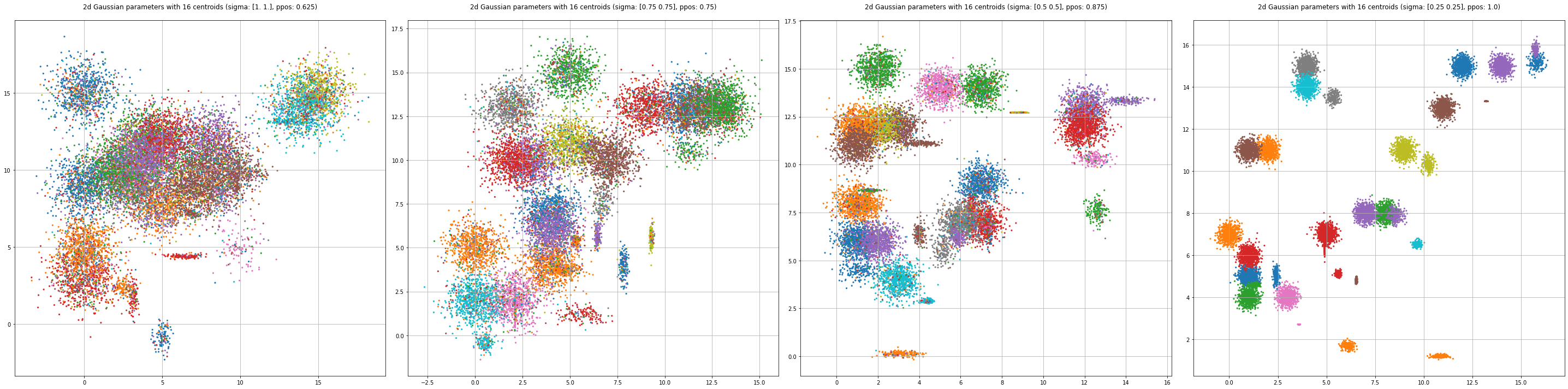
A good contrastive loss function should be able to produce values that correlate to the compressive-contrastive qualities of the latent space representations. Hypothetically, this should hold true even if the latent space is just generated from a random process. I thought this would be a good area to experiment in, so I wrote some code to generates \(n\) samples from \(k\) clusters in a \(d\)-dimensional space.
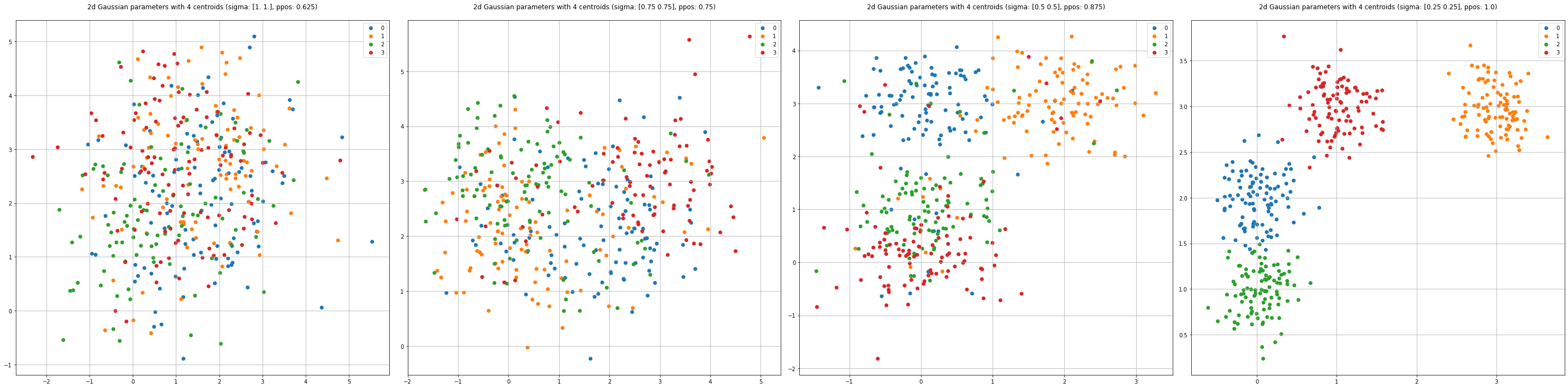
Another element in my program is the addition of discrete biases and label corruption to each classes’ Gaussian.
Experimental Approach
My strategy was to compare the pairwise distance matrices for each L2, FLD, and MCR\(^{2}\) over increments of linear separability in the generated data. As, the iterations increase from [0/end], we should expect to see an increase in contrast between the diagonal of the matrices and their upper/lower triangles. This is just to say that the loss function measured between just two pairs of classes should show good separation. Ultimately, we should expect to see the total loss function monotonically decrease over the course of iterations. The interesting thing will be to see what changes here as the number of dimensions increase.
Experimental Results
Below is the log output from one iteration of the experiment, the full script can be accessed here.


Observations
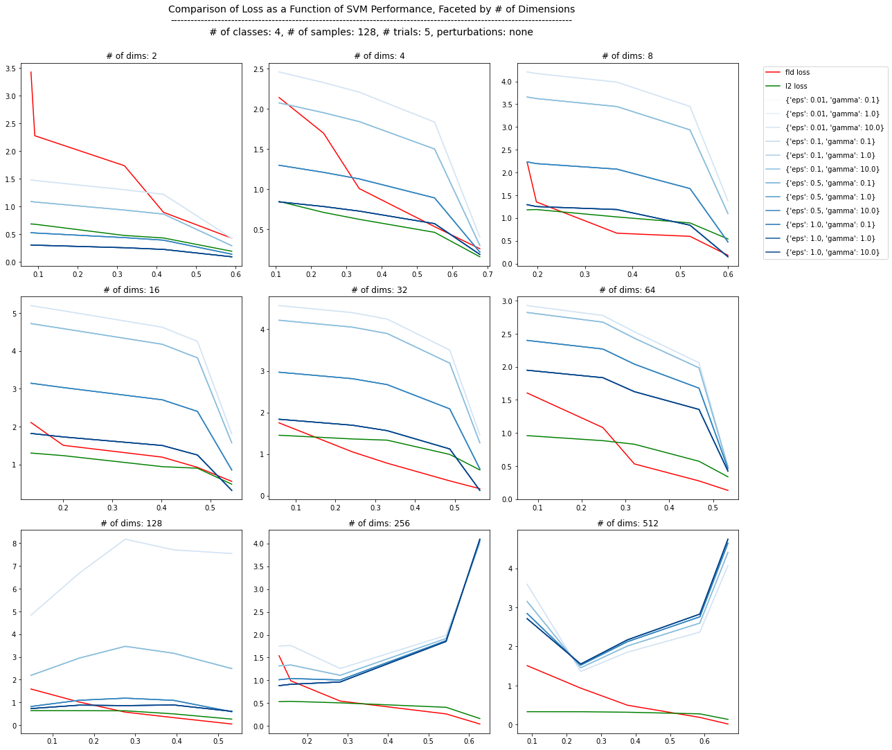
I plotted the overall loss functions over all iterations for each # of dimensions below. The x-axis tracks the overall class prediction accuracy for an SVM classifier, which explains the slight back-tracking in these plots. The y-axis is a standardized version of the true loss function, just so everything fits on the same scale. If these loss functions are good indicators of linear separability, there should be a downward trend over the iterations in the experiment, and this behavior should stay true more or less as the # of dimensions increase. Interestingly, we start to see some noisyness in the MCR\(^{2}\) los functions when we surpass 64 dimensions. In these data, it seems that for MCR\(^{2}\) the within-class/between-class components stay more or less the same. Since we know that we’re increasing the linear separability of the classes, we should expect to see the compressive loss decrease, and the contrastive loss increase. There may be some important parameter to tune with respect to the number of dimensions, or maybe even a bug in implementation. The L2 (annotated as “euclidean” here) also looks a little wonky in higher dimensions. However, if we look back up at the experimental output, the distance matrix for the euclidean loss shows the increase in diagonal vs. upper/lower triangle contrast that we’re expecting better in higher dimensions than the FLD and MCR\(^{2}\) matrices.
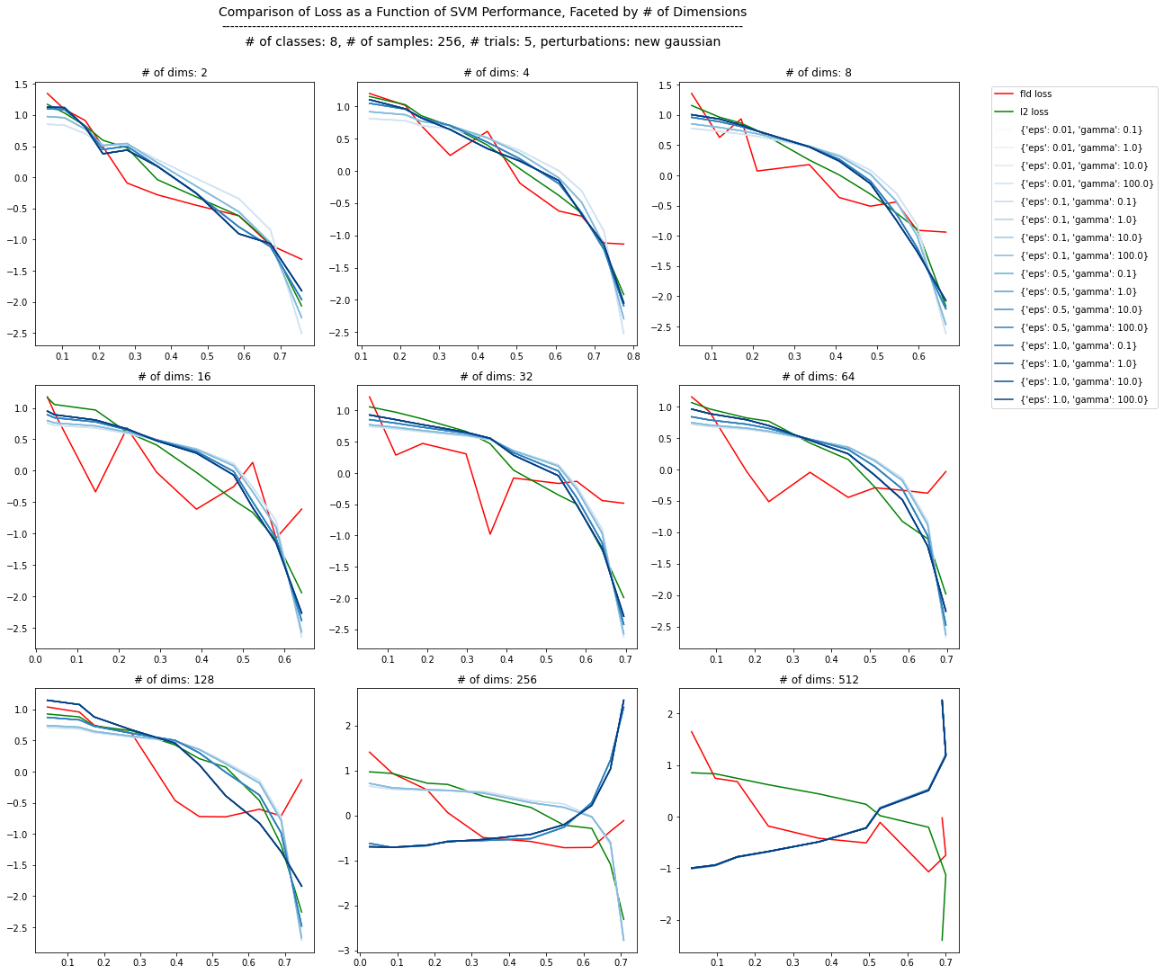
Increasing the number of classes yields similar results.
Discussion
It’s very possible at this point there is either some kind of implementation error in my MCR\(^{2}\) loss function, or an incorrect assumption being made about the data. It’s common to see one or more of these kinds of problems when doing R&D. However, I think this general method of simulating data that is more or less what the objective function seeks is still useful for inspecting how a loss function behaves.
Thanks for reading 🤙!
Acknowledgements
Thanks to the authors of the MCR\(^2\) paper, and @ryanchankh for the open-source implementation.