Introduction

Two critical parts of researching air pollution are understanding the source of a pollutant, and understanding who and what is affected by it. From a researcher’s standpoint, determining pollution sources can be difficult because publicly available data on the locations of energy production and dispersion of energy consumption isn’t abundant. Fortunately, satellite images of atmospheric composition are pretty easy to find. They usually are composed of an estimate of chemical concentration in a lat/lon coordinate system. It seems like a useful goal, or at least an interesting experiment, to try and tease apart the source locations and source types from a signal like this. To do this, a mathematical operator called divergence can be used to trace the outward flow of energy- in this case the concentration of a pollutant- back to a source. In this post, I talk about the mathematical idea of divergence, and share a project I worked on that visualizes an estimatation of pollution sources using divergence.

Divergence

Divergence is a scalar function that measures the amount of outward flux at a point in a vector space. It is well illustrated by the concept of water flowing from a faucet, into a bathtub, and down a drain. The water flows outward from a source- the faucet, and inward into a sink- the drain. The spatial system representing the bathtub has positive divergence at it’s source point, and negative divergence at it’s sink. At points in the system where water passes through, i.e. the same amount of water that passes into the point also passes out of it, it’s divergence is zero. Divergence in a system is zero everywhere except for where flux is entering or leaving the system.

Mathematically, there are various ways of defining divergence, but a very simple way divergence can be computed is by taking the sum of the gradients in each direction of the coordinate space. In the equation below, I’ve notated the dimensions as \(x, y, t\) because the coordinate system I am working with has two spatial directions and one time dimension.

\[\text{div F} = \frac{\partial F_{x}}{\partial x} + \frac{\partial F_{y}}{\partial y} + \frac{\partial F_{t}}{\partial t} \tag{1}\]

Since we’re interested in arriving at some estimate of the sources and sinks of the air pollution dataset, we’ll compute the gradient from the data, and estimate the divergence through equation 1. Recalling that the gradient is a vector field of partial derivatives, each point \(p\) in the gradient space corresponds to a vector containing the partial derivates for all \(d\) dimensions:

\[\nabla f(p) = \begin{bmatrix} \text{ } \frac{\partial f}{\partial x}(p)\\ \frac{\partial f}{\partial y}(p)\\ \frac{\partial f}{\partial t}(p)\\ \text{ } \end{bmatrix} \tag{2}\]

So for any point \(F = (F_{x}, F_{y}, F_{z})\), we just compute the dot product between \(F\) and \(\nabla f(p)\):

\[div F = \nabla f(p) \cdot F \tag{3}\]

In the context of computing these values from real data, each of these partial derivatives is computed via the difference quotient, where \(h\) in this discrete context is a step-size in reference to our coordinate space:

\[\frac{f(x + h) - f(x)}{h} \tag{4}\]

This is the very fundamental idea behind gradient computation, but it can get a lot more sophisticated. For a precise explanation on how the gradient is approximated from real data in NumPy’s gradient() function, I recommend reading their documentation page.

Air Quality and Population GIS Data

The air quality data I used came from the SILAM Global Air Quality forecast, produced by the Finnish Meteorological Institute [1]. These data are an estimate of chemical concentration in ug/m3 for a variety of known pollutants.

As I researched for this experiment, it seemed useful to know how pollution concentration correlates with population density. Should we expect to see pollution sources generally sequestered from population centers, as may be the case with oil refineries in Canada or Alaska? Or is it common to see high pollution concentration in populous cities, or spanned over sparser populations? I incorporated population density data from CIESIN+Meta, and approximated a mapping between that coordinate system onto the air quality dataset coordinates.

Estimating Divergence

When the sum of the gradients in all dimensions at a point is positive, it means that there is an aggregate net positive change from that point outwards. This is a case of positive divergence at a point.

For this problem, the dimensions we are dealing with are the lat, lon and time dimensions. To give some visualization, I created a .gif of the gradient flow of NO2 pollution for a single day. The animation runs backwards, hopefully giving a very rough idea of pollution flowing back into its source. Calculating divergence is something like taking the sum of this animation for any single point.

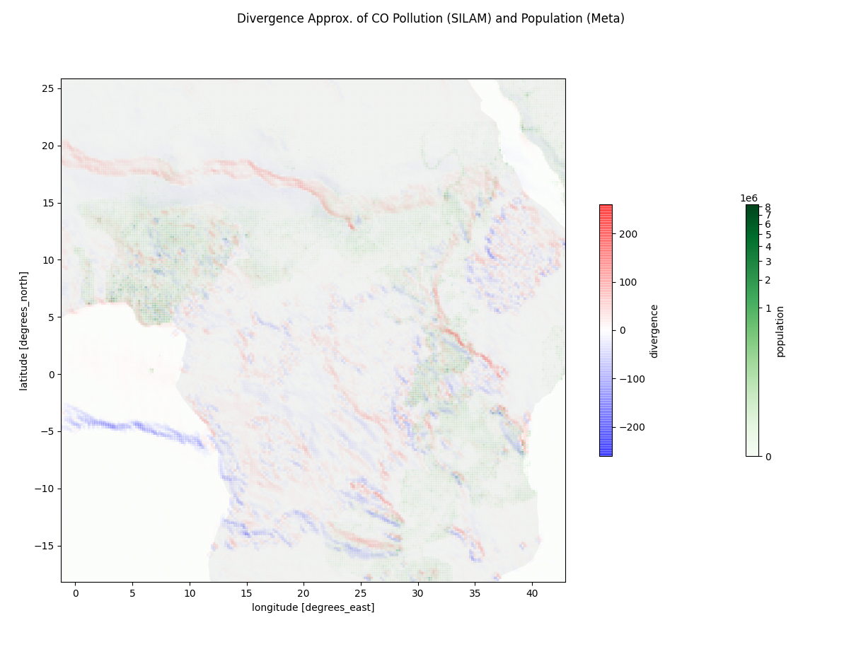
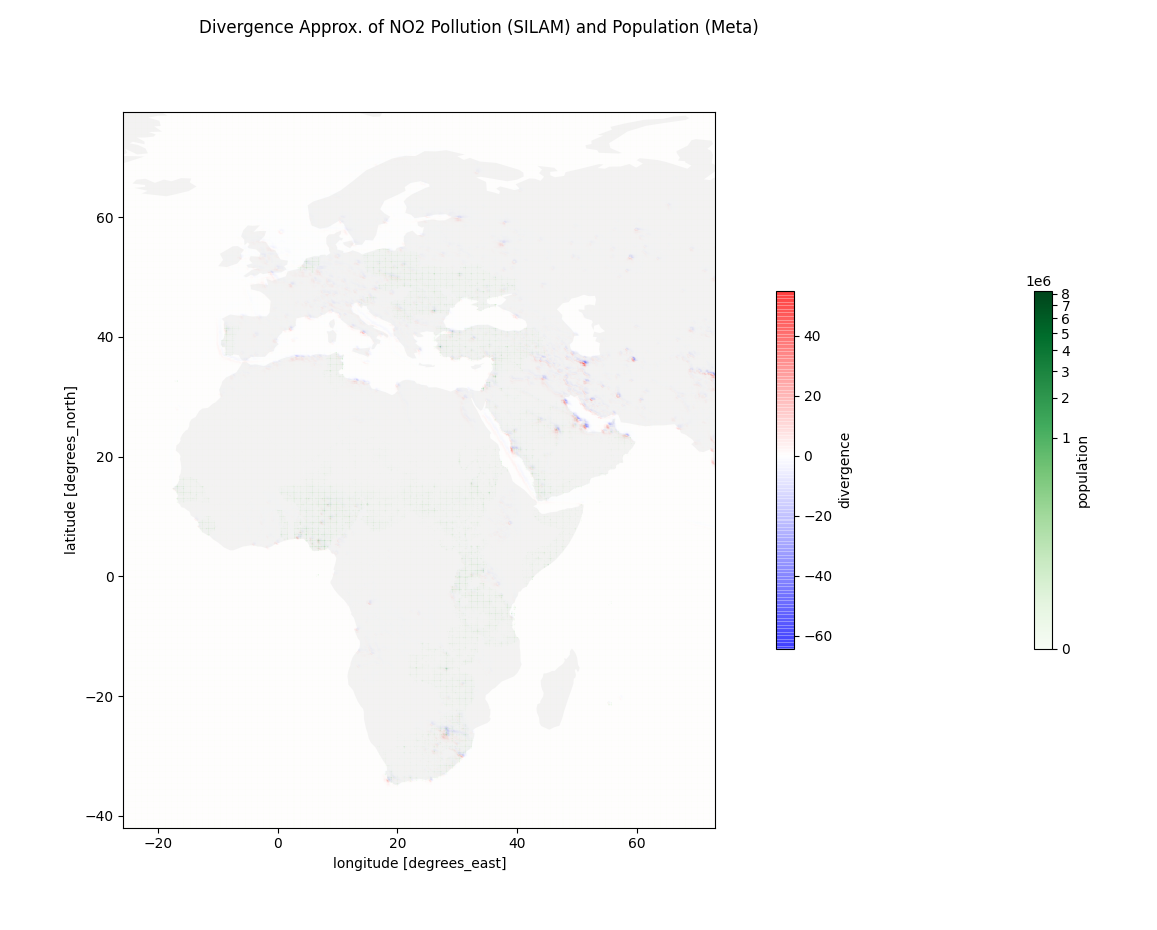
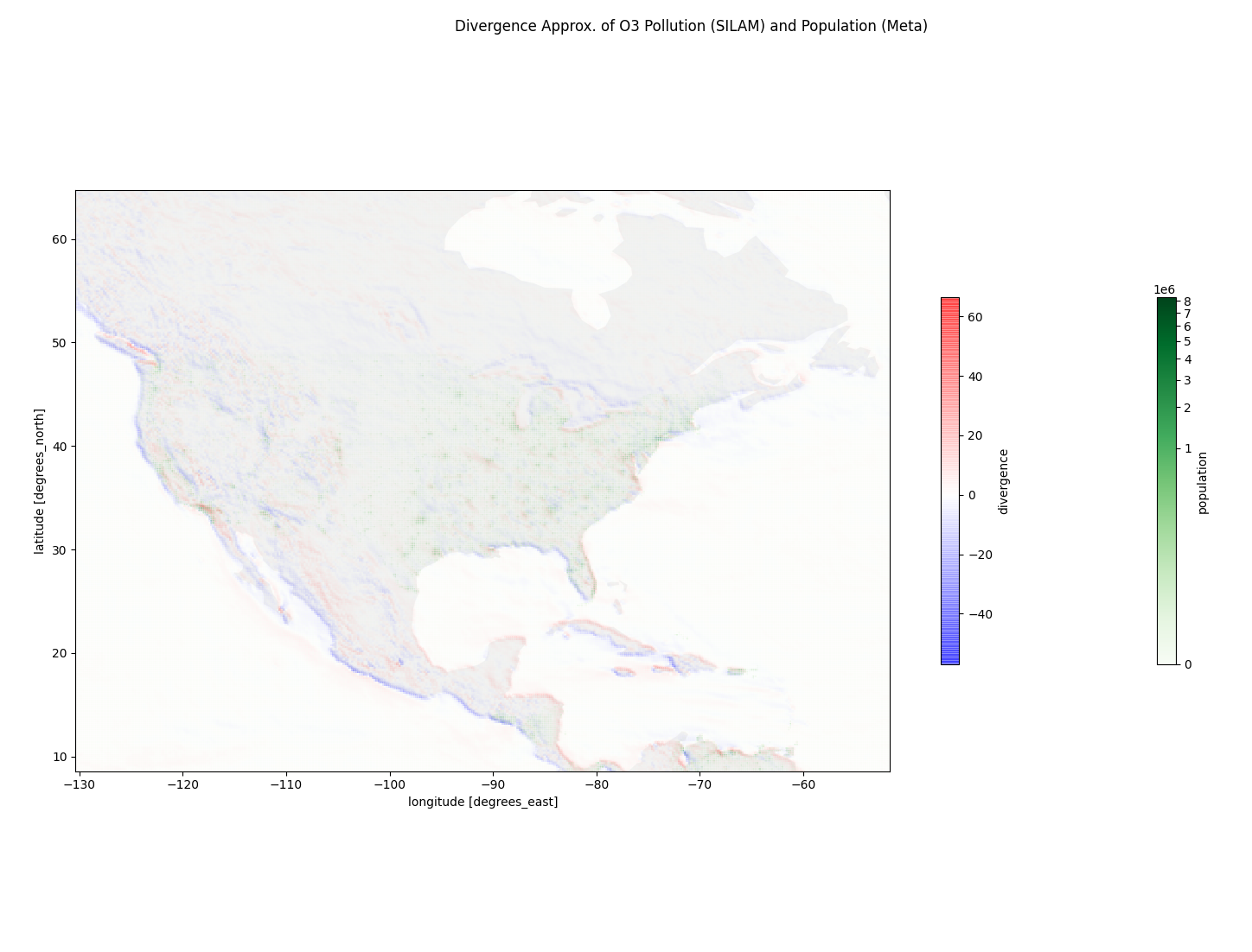
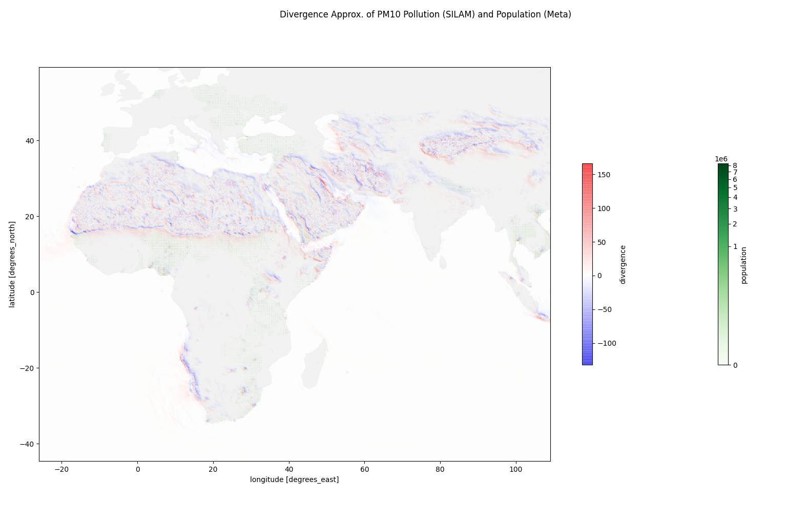
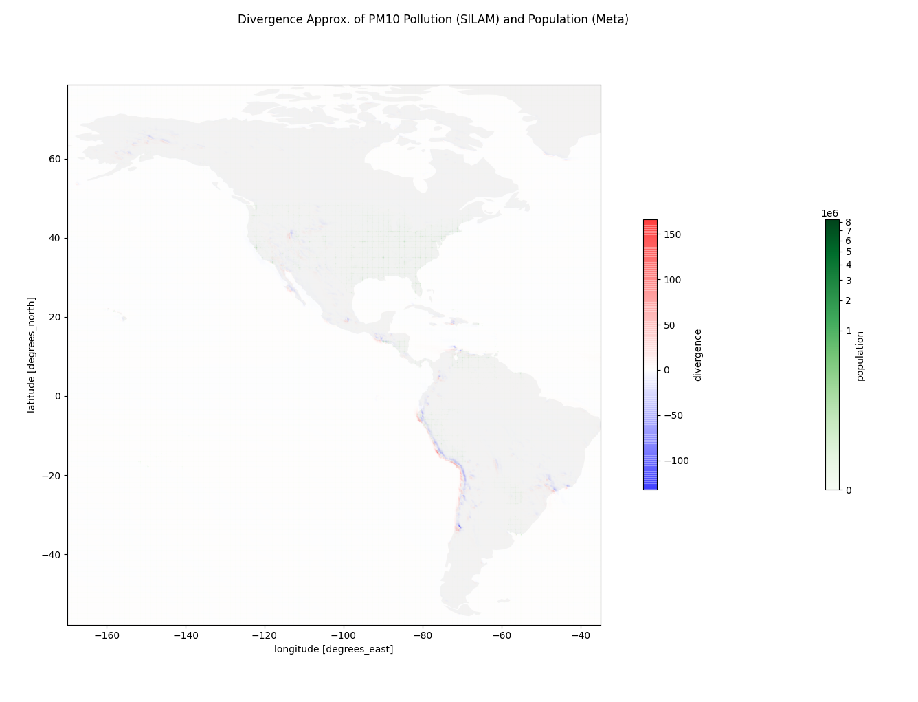
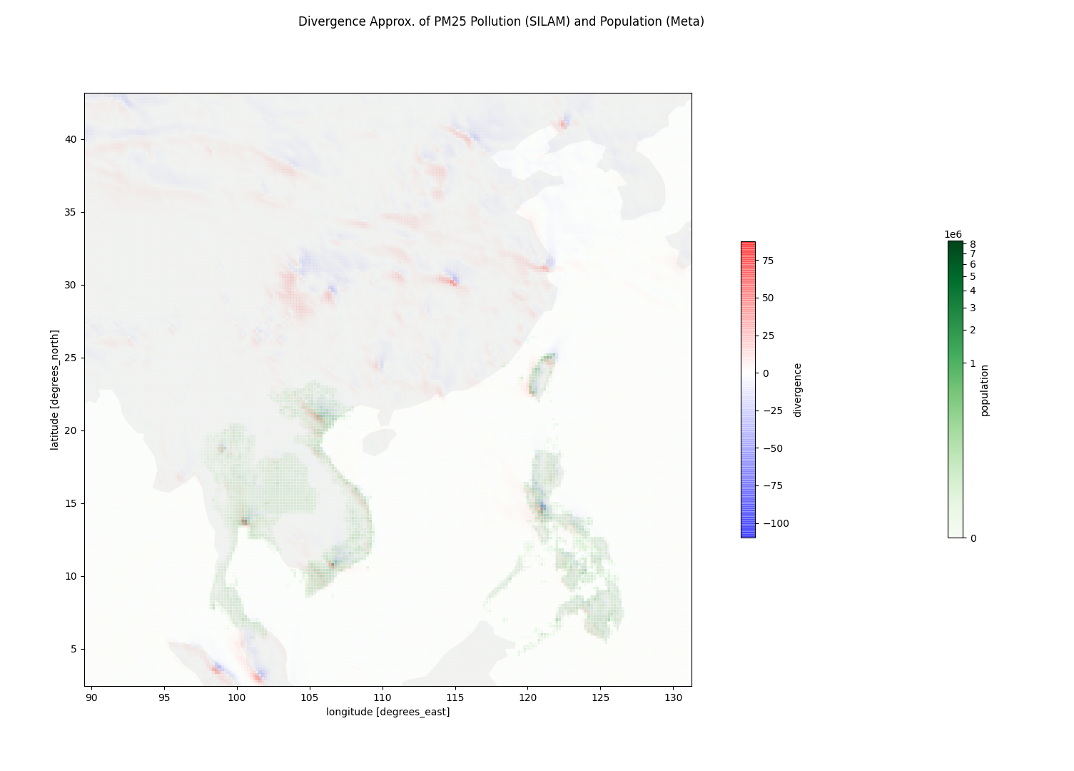
The divergence estimation programs can be found at https://github.com/deanjgoldman/asdi-aq-view/tree/master/scripts. Below are some screenshots of points of interest:

Observations

It would be great to merge this data with some complete data around population density, lifespan, climate, energy production, and energy consumption. There seems like a multitude of opportunities, a few that come to mind are:

• Attributing the proportion of pollution to various energy production/consumption activities, localized or dispersed.
• Predicting the amount of homes that produce energy by burning wood or biomass.
• Predicting the expected decrease in pollution given some change in energy mix models.
• Quantifying the expected effect on healthy lifespans for populations living in high pollution areas. Using this to build a model to guide energy technology, while minimizing impact on people’s health.
• Identifying highly populous areas with the least pollution.

References

[1] SILAM Air Quality was accessed on July 27, 2022 from https://registry.opendata.aws/silam.

[2] High Resolution Population Density Maps + Demographic Estimates by CIESIN and Meta was accessed on July 27, 2022 from https://registry.opendata.aws/dataforgood-fb-hrsl. Meta and Center for International Earth Science Information Network - CIESIN - Columbia University. 2022. High Resolution Settlement Layer (HRSL). Source imagery for HRSL © 2016 Maxar. Accessed 27 07 2022.