Energy Flow in a Graph Through Message Passing
26 Sep 2022 - Dean Goldman
Graphs
This post will assume some basic knowledge of what graphs are, but just to lay out the general theme and some notation I’ll be using, this is an example of a graph, specifically a multidigraph:
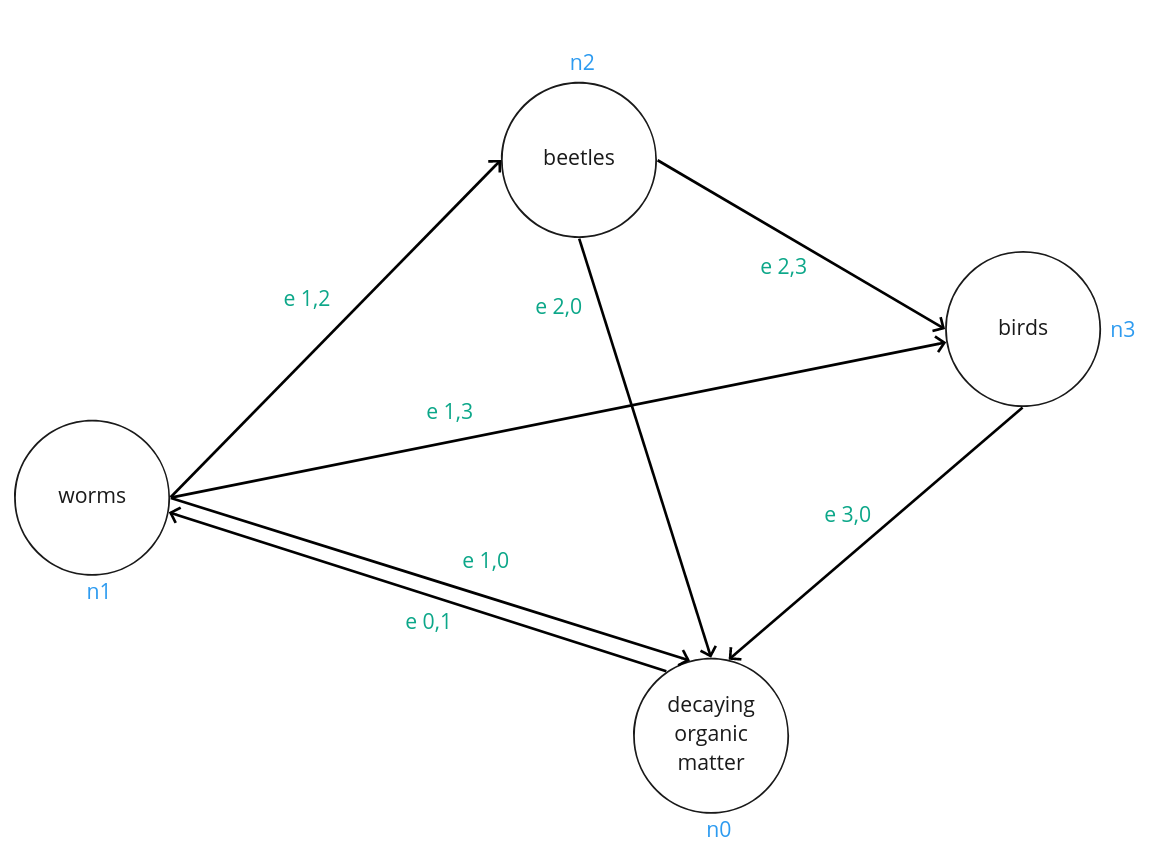
This graph is a simplified representation of a food web, a representation of certain taxonomies consuming others. Notice that all taxonomies are connected to ‘decaying organic matter’, which is the process of death and decompositon. That node also sends outward to the node labelled ‘worms’, indicating that worms consume decomposed organic matter. This is an example of a graph with multiple directed edges, meaning that it is possible for node 0 to receive energy from node 1, and simultaenously possible for node 0 to give energy to node 1. To understand the flow of energy through a graph is commonly done through an adjacency matrix:
\[A = \begin{bmatrix} e_{0,0} & e_{0,1} & e_{0,2} & e_{0,3} \\ e_{1,0} & e_{1,1} & e_{1,2} & e_{1,3} \\ e_{2,0} & e_{2,1} & e_{2,2} & e_{2,3} \\ e_{3,0} & e_{3,1} & e_{3,2} & e_{3,3} \end{bmatrix}\]An adjacency matrix is a square matrix that represents connections in a finite graph. Each element of the matrix represents the connection between a pair of nodes in the graph. Values of an adjacency matrix can be denoted in binary: indicating a connection (1) or no connection (0), which is often referred to as an incidence matrix. Values can also be the amount of energy flow between nodes.
In undirected graphs, nodes are connected by edges that do not have a particular direction. In this case, adjacency matrices are symmetric, since the flow across the edge from \(i\) to \(j\) is identical to the flow across the edge from \(j\) to \(i\). In directed graphs the adjacency matrix is not necessarily symmetric; the ordering of \(i,j\) or \(j,i\) will matter since that order will determine the direction of the flow between the two nodes. In some directed graphs, energy flows between nodes in only one direction, this is known as a simple directed graph. An easy example is a sequential set of tasks, where one task must take place and pass on whatever task output to the next task. However in the case of our food web example- a multidigraph- energy flows in both directions. In either case, for adjacency matrices of directed graphs, one dimension of A will correspond to the energy flowing out of a node, and another will correspond to the energy flowing in to a node. And as usual, a zero value indicates no energy flow.
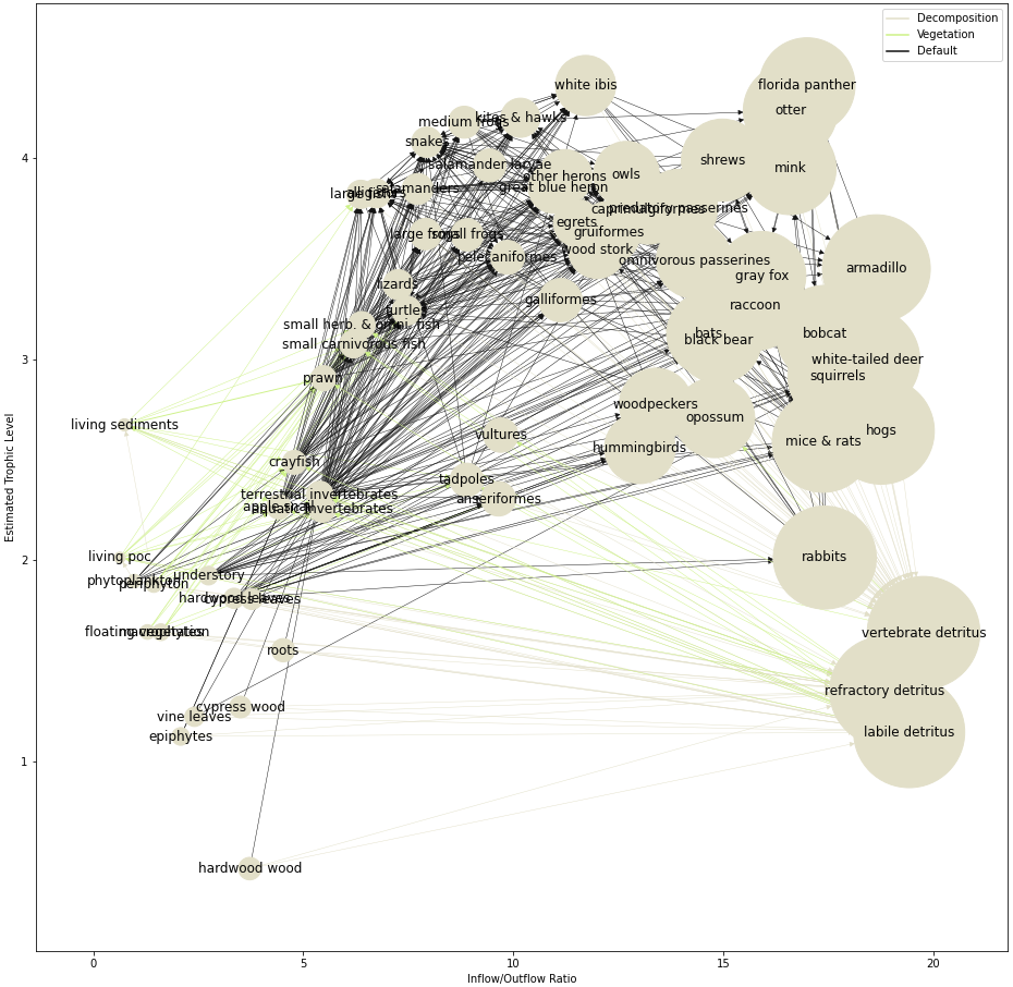
Example Dataset: South Florida Ecosystem Food Web
This dataset is an estimate of carbon exchange between taxonomies in the ecosystems of South Florida. Each node represents a taxonomy- a component of the ecosystem- and each edge represents the transfer energy between components, i.e. “Who eats whom, and by how much?” [1].
1. Computing Feature Changes Through Time
If we want to know what a set of node features will be after one state transition, we can compute this through what’s called a graph convolution. In linear algebra terms, this is just the dot product between the set of node feature vectors and the weighted graph adjacency matrix:
\[N_{t=1} = A \cdot N_{t=0}\]For the South Florida Ecosystem Food Web, the only feature we’re measuring is “biomass”, so we can represent this 1-d feature vector with a barplot:
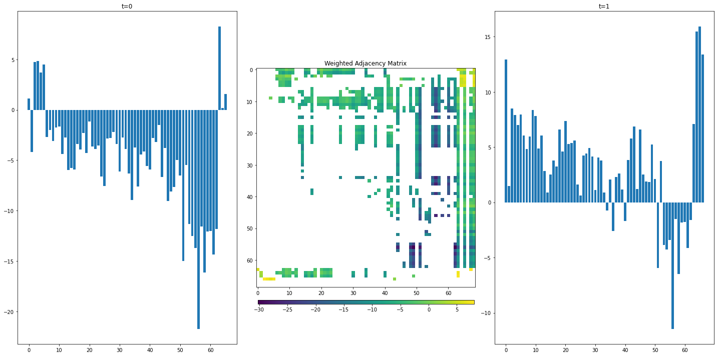
The weighted adjacency matrix allows us to pass energy from nodes at timestep \(t=0\) to it’s neighbors, producing a feature set at timestep \(t=1\). We’ve essentially simulated an exchange of energy between compartments in the ecosystem. Graph convolutions are a limited case of what is known more generally as message passing.
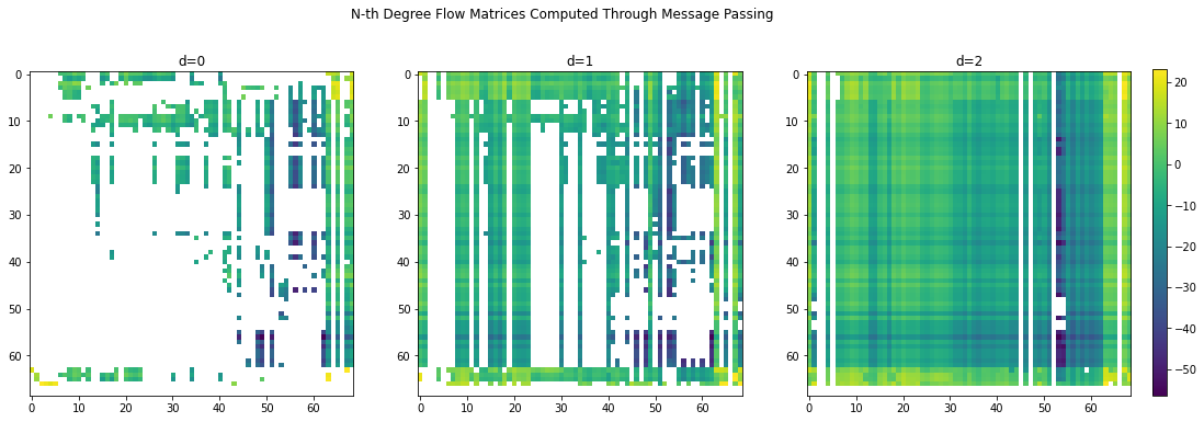
1. Computing Connectivity
In the Cypress Ecosystem example, we can see that the “white ibis” feeds on “tadpoles”, and the “gray fox” feeds on the “white ibis”. If we wanted to know how much biomass flows from “tadpoles” to “gray fox” in total (either through the “white ibis” or other relationships), we can compute a second-order adjacency matrix, which tells us the energy flow for second-order connections in the graph.
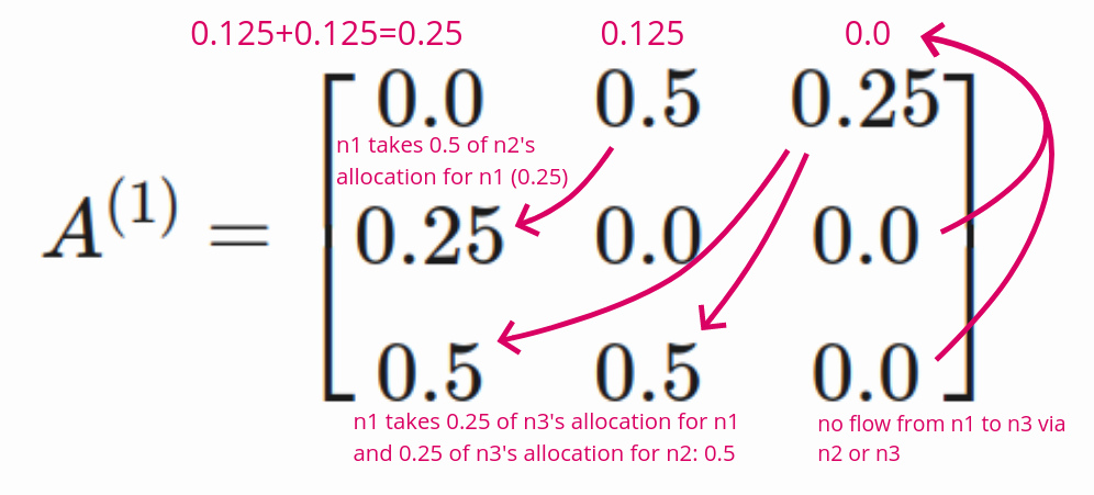
\[A^{(2)} = A^{(1)} \cdot A^{(1)} \\\]Personally, this is a little hard to intuit, but it can be visualized. Let’s start with a very simple weighted adjacency matrix:
\[A^{(1)} = \begin{bmatrix} 0.0 & 0.5 & 0.25 \\ 0.25 & 0.0 & 0.0 \\ 0.5 & 0.5 & 0.0 \end{bmatrix}\] \[A^{(1)} \cdot A^{(1)} = \begin{bmatrix} (0.0 * 0.0 + 0.5 * 0.25 + 0.25 * 0.5) & (0.25 * 0.0 + 0.0 * 0.25 + 0.0 * 0.5) & (0.5 * 0.0 + 0.5 * 0.25 + 0.0 * 0.5) \\ (0.0 * 0.5 + 0.5 * 0.0 + 0.25 * 0.5) & (0.25 * 0.5 + 0.0 * 0.0 + 0.0 * 0.5) & (0.5 * 0.5 + 0.5 * 0.0 + 0.0 * 0.5) \\ (0.0 * 0.25 + 0.5 * 0.0 + 0.25 * 0.0) & (0.25 * 0.25 + 0.0 * 0.0 + 0.0 * 0.0) & (0.5 * 0.25 + 0.5 * 0.0 + 0.0 * 0.0) \end{bmatrix}\] \[A^{(2)} = \begin{bmatrix} 0.25 & 0.125 & 0.0 \\ 0.0 & 0.125 & 0.0625 \\ 0.125 & 0.25 & 0.125 \\ \end{bmatrix}\]It can be shown that the new values for the first row (\(N_{0}\)’s outgoing flow) is the amount of energy that passed through \(N_{0}\) to it’s neighbors, and from those neighbors back to \(N_{0}\), which is then distributed in proportion to the original flow values.
In the case of the Food Web example, higher degrees of the adjacency matrix rerpresent more and more interconnectedness, meaning at some level, most species are consuming matter that at one point belonged to any of the other species: