Finding a Multivariate Gaussian Probability Distribution For Discrete Points
08 Feb 2023 - Dean Goldman
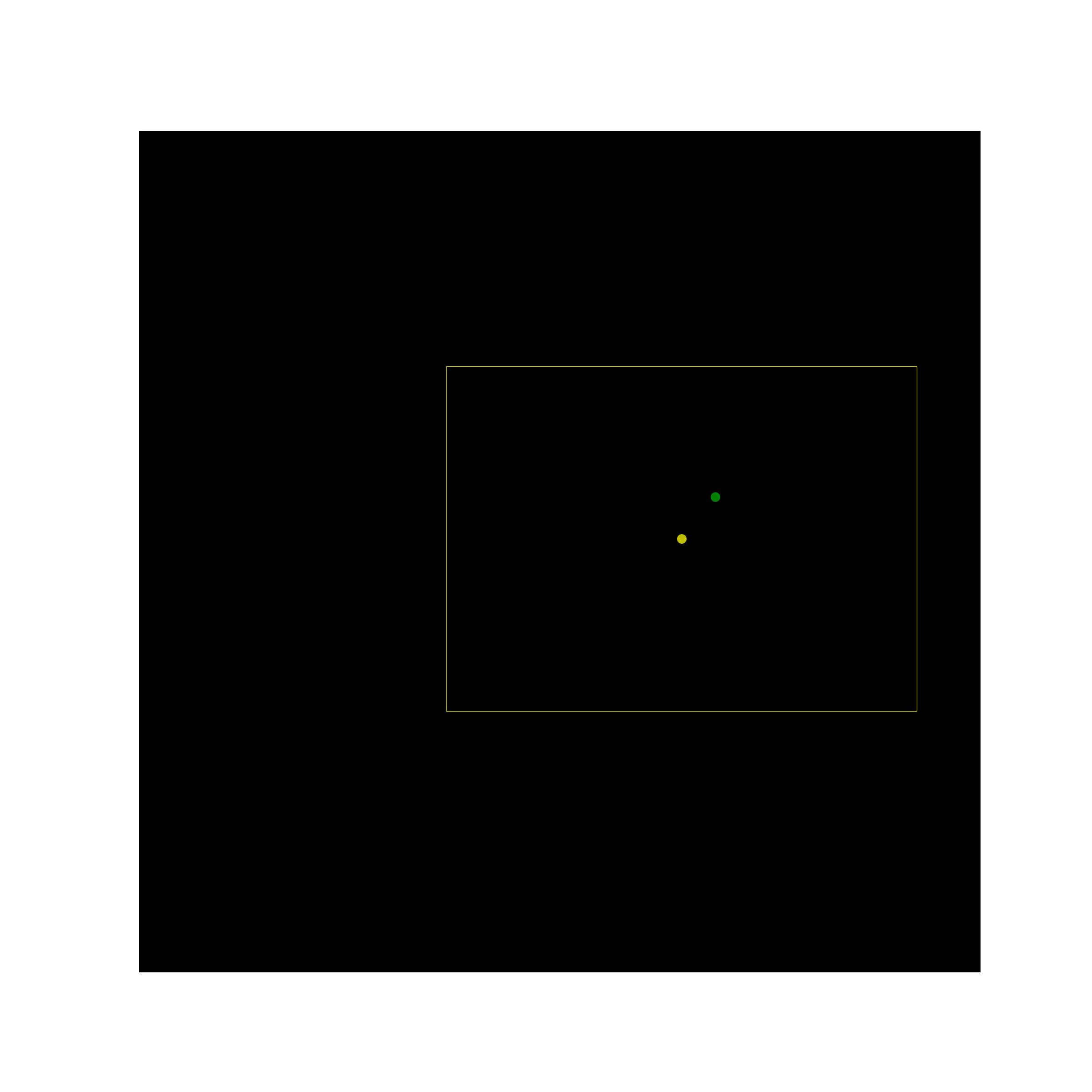
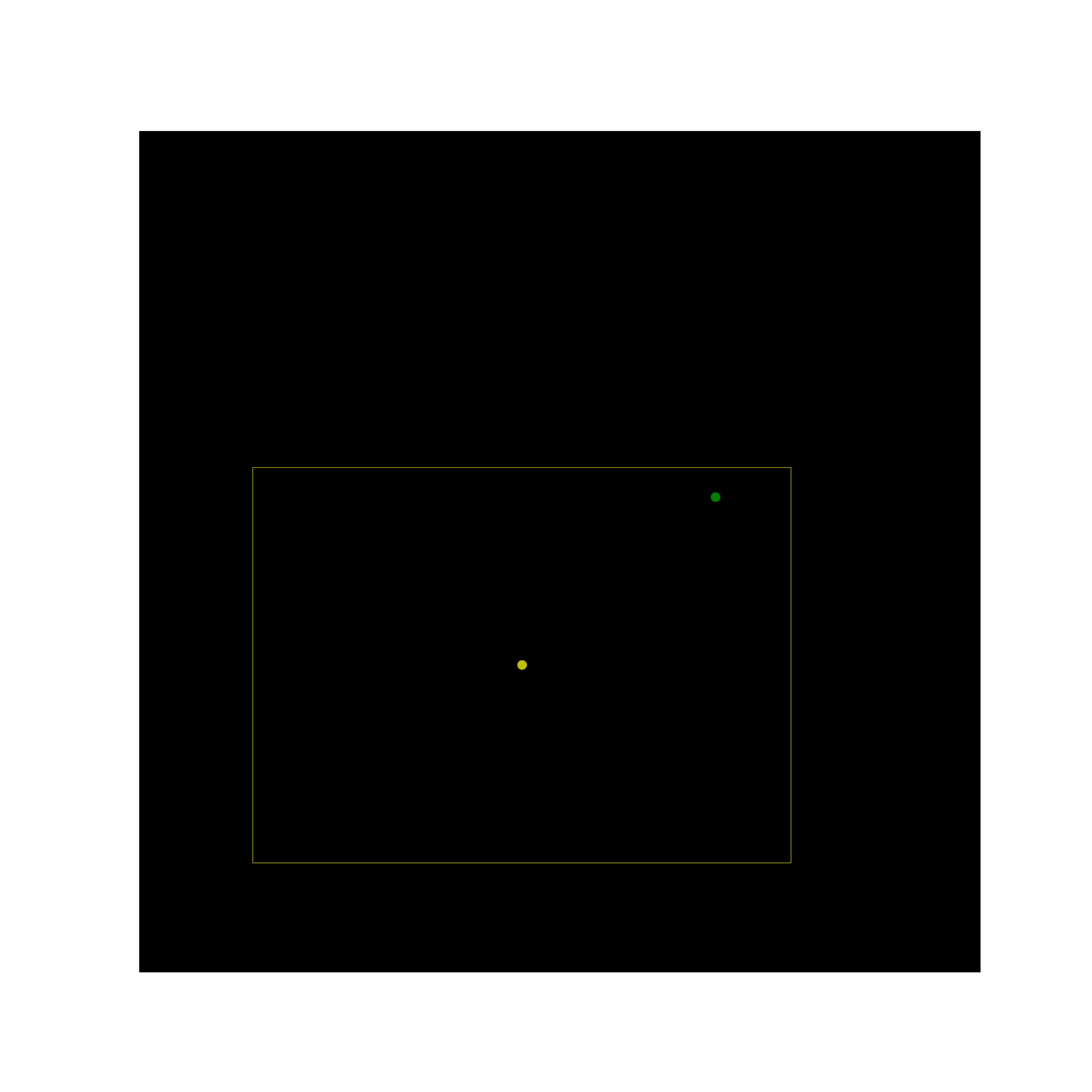
I recently worked on a project where our goal was to find some measure of probabilistic affinity between a sample point and a box in 2d space. We framed the problem as finding the probability that our sample point belongs to a 2d Gaussian distribution parameterized by the box center point, and standard deviations which we could derive from the box width and height. So for the following two box and point pairs, we would have a high and low probability assigned:
Defining a Probability Distribution
Finding these probabilities involves utilizing the probability density function for multivariate Gaussians.
\[f(x \mid \mu,\Sigma)=(2\pi)^{-\frac{k}{2}} det(\Sigma)^{-\frac{1}{2}} e^{(-\frac{1}{2}(x-\mu)^T\Sigma^{-1}(x-\mu))}\]One thing to note though is that the coordinates in this 2d space are discrete, and the pdf is only defined for continuous distributions, and is also a probability density, not a probability. There are a number of methods for finding a probability, including computing an interval over \(f(x\mid \mu, \Sigma)\). But the simplest, and probably fastest method I found was to use just a particular component of the pdf- the Mahalanobis distance \(r\).
\[r^2 = (x-\mu)^T\Sigma^{-1}(x-\mu)\]Reading the definition of the Mahalanobis distance, its use seems completely appropriate:
The Mahalanobis distance is a measure of the distance between a point P and a distribution D, introduced by P. C. Mahalanobis in 1936 [1].
So in our case, we’re looking for the probability that a random sample would have distance \(r\) from the mean of distribution parameterized by \(\mu, \Sigma\), or the probability of a pair \((p, D)\) with Mahalanobis distance \(r\).
What is very convenient about the Mahalanobis distance, is that when it is expressed as a distribution of squares, or \(r^2 \sim R\), we can characterize that as a distribution of the sum of square deviations from the mean. This happens to be the definition of the chi-squared distribution. So we can characterize the distribution of the Mahalanobis distance by the chi-squared distribution:
\[r^2 \sim \chi^2_{k}, k=2\]Two things left: the first thing is that chi-square distributions are defined for continuous space. So we still need to integrate that into a probability. Luckily, the cumulative density function \(F(x,k), k=2\) is much easier to compute. But this is actually the probability that a squared distance will be less than \(r^2\), which would assign small probabilities to very close distances and vice-versa. We are actually interested in the inverse of that, so we instead use:
\[1 - F(x,k), k=2\]Without going into too much detail, the cdf of \(\chi^{2}_{k},k=2\) is defined simply as [3]:
\[F(x; 2)=1-e^{-\frac{x}{2}}\]So we have the following, very simple equation that will express our desired probability:
\[P(R \gt r^2) \sim 1-F(x; 2)=1-(1-e^{-\frac{x}{2}}) = e^{-\frac{x}{2}}\]Note: \(x\) and \(r^2\) represent the same value here.
Implementation with Specific Data Structures
For this particular case, the “distribution” we are sampling from is approximated by what we are actually measuring around, a box. To approximate a Gaussian distribution defined by a box, we can use the box centroid as \(\mu\), and use the box width and height to derive a standard deviation \(\sigma\) in both \(x,y\) directions. If we follow the 68-95-99 rule, three standard deviations from \(\mu\) should give us 99.7% of our data. This is analogous to saying that at three standard deviations away from \(\mu\), we are quite close to the edge of our box. So we can make a quick approximation of \(\sigma\) by halving \(w,h\) to start at the box centroid, and divide by three: \(\sigma=box_{w,h}/6\) (this is also parameterizable). We don’t have any covariances in the upper or lower triangles of \(\Sigma\), because we’re dealing with a box, not a population. Plugging our sample point \(s\) into this equation of the Mahalanobis distance, we get:
\[r^2= \begin{bmatrix} (s_{x} - \mu_{x}) \\ (s_{y} - \mu_{y}) \\ \end{bmatrix} \begin{bmatrix} \sigma_{x} & 0 \\ 0 & \sigma_{y} \\ \end{bmatrix}^{-1} \begin{bmatrix} s_{x} - \mu_{x} & s_{y} - \mu_{y} \\ \end{bmatrix}\]We can now use the cumulative distribution function of the chi-squared distribution:
\[F(r^2; 2)=1-e^{-\frac{r^2}{2}}\]Results
The plots below display some examples of this implementation. A multivariate Gaussian pdf has been plotted at discrete points in the coordinate space as a helpful sanity check, alongside a computation of \(F(r^2;2)\).
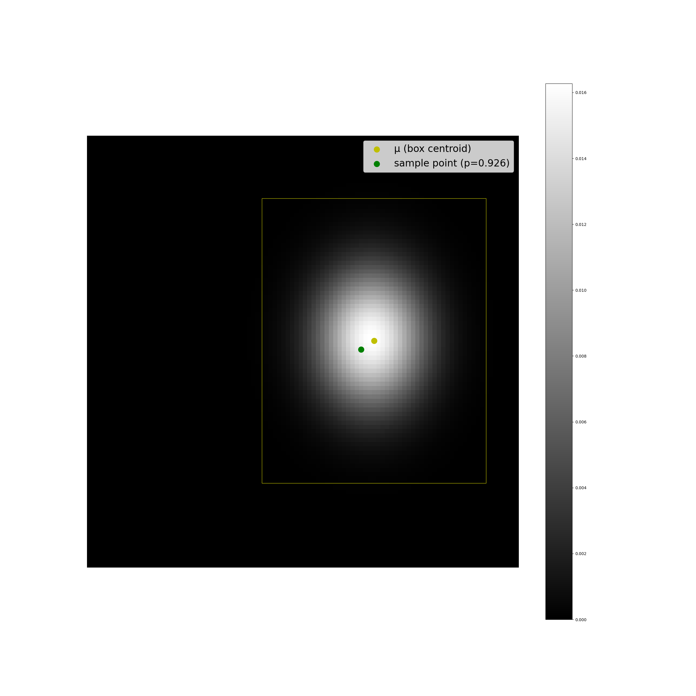
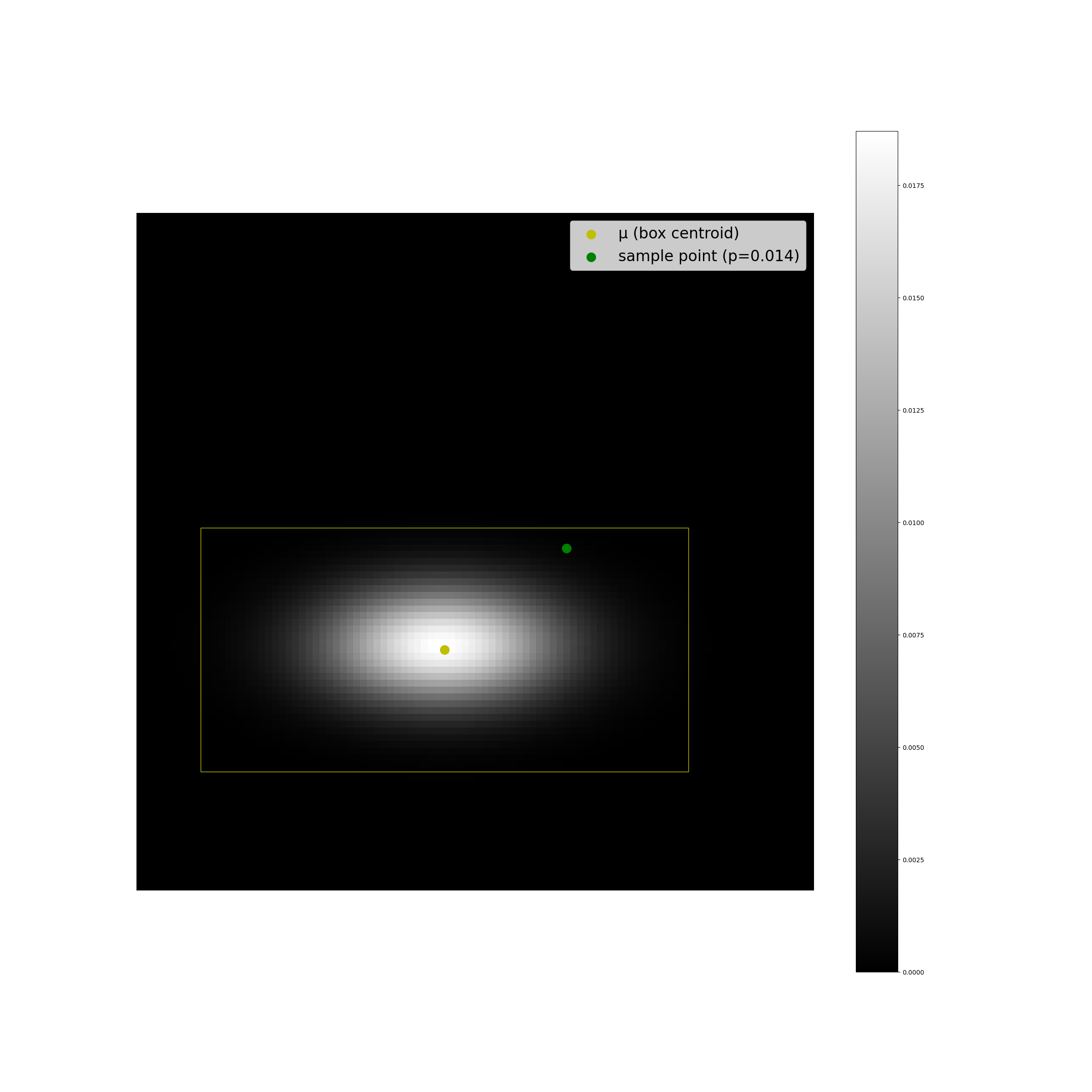
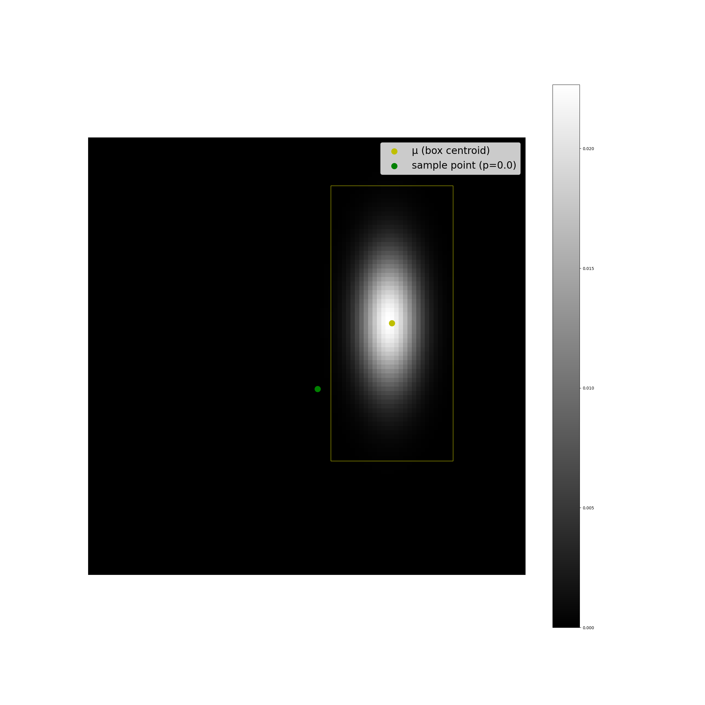
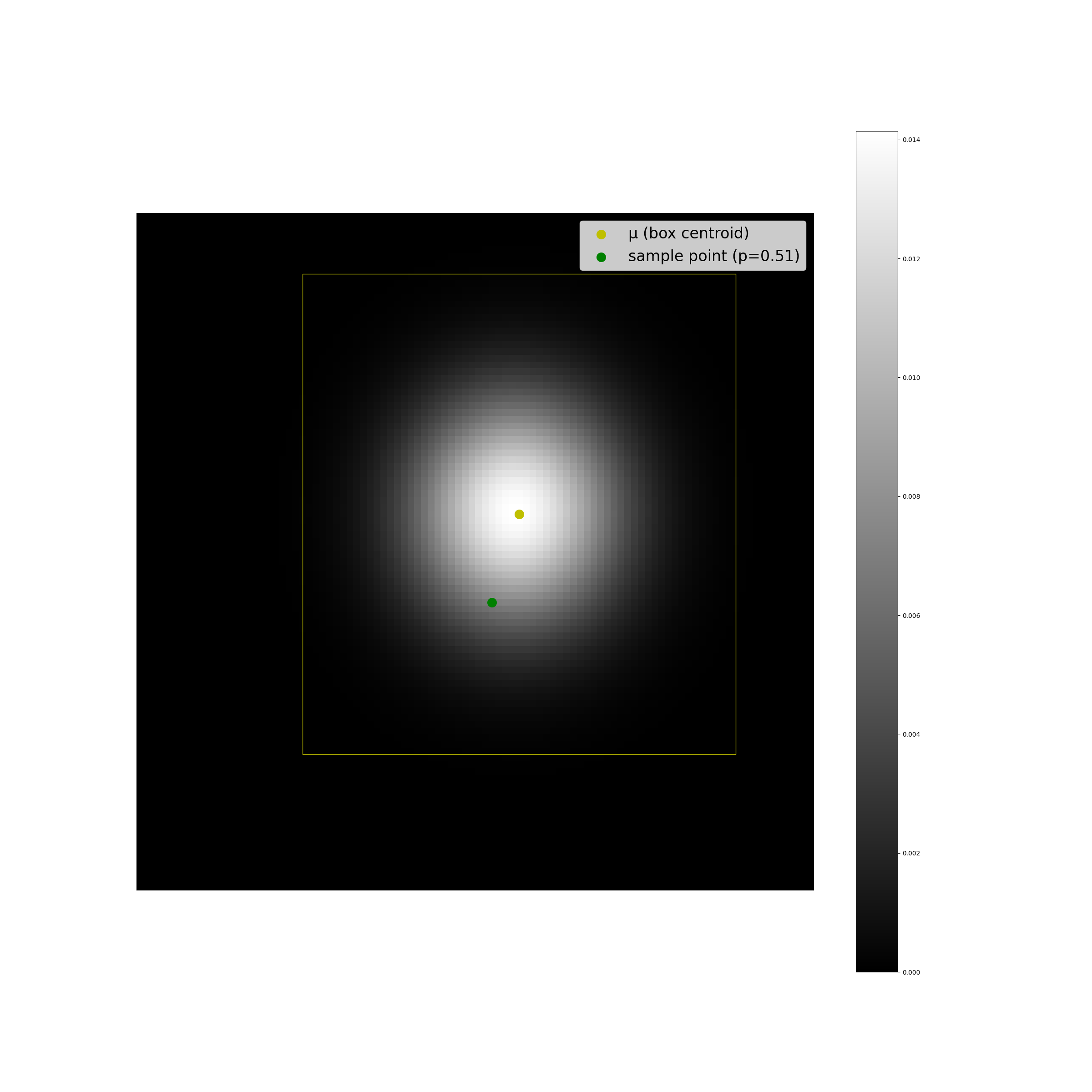
We can see that the results look as we expect they should, and the code is suprisingly simple.
import numpy as np

def cdf_2d_gaussian_from_box(x, mu, sigma):
    '''
    Computes a probability of a point x being sampled from a
    2d standard normal distribution D defined by mu, sigma.
    Supports vectorized inputs.

    Arguments:
      x: sample points, array(m, 2)
      mu: box centroids, array(n, 2)
      sigma: box wh, array(n, 2)

    Returns:
      p: probability of sampling x from D, array(n, m)
    '''

    # compute mahalanobis distance
    dist = x - np.expand_dims(mu, 1)
    r2 = (dist[:, :, 0] / np.expand_dims(sigma[:, 0], 1))**2 + \
        (dist[:, :, 1] / np.expand_dims(sigma[:, 1], 1))**2

    # compute chisq cdf
    p = np.exp(-r2/2)

    return p
Discussion
It was fun to dive into a pretty dense equation like a multivariate Gaussian pdf and pull out exactly what was needed for this particular problem. Understanding precisely how each input term relates to the underlying mathematics reduced the need for a bunch of extra computation, which is great. This could definitely be extended to higher dimensions, and to real distributions, as I’ve seen around in some open-source repos and other blogs.