Variable Analysis for Improving a Regression Model
24 Aug 2023 - Dean Goldman
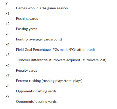
The Table B1 dataset published in Introduction to Linear Regression Analysis, Montgomery, D.C., Peck, E.A., and Vining, C.G. (2001) [1] has 28 observations of team statistics in the 1976 National Football League. These observations include statistics of the number of games won, rushing yards, passing yards, opponent’s rushing yards, opponent’s passing yards, punting, field goals, turnovers, and penalties over the course of a 14 game season. The stated problem is to predict the number of games won in the season, using some set of the given variables. The variable information is given in [2]:
As a quick snapshot, a pairplot of the y ~ x can show the spread and correlation coefficients of our variables:
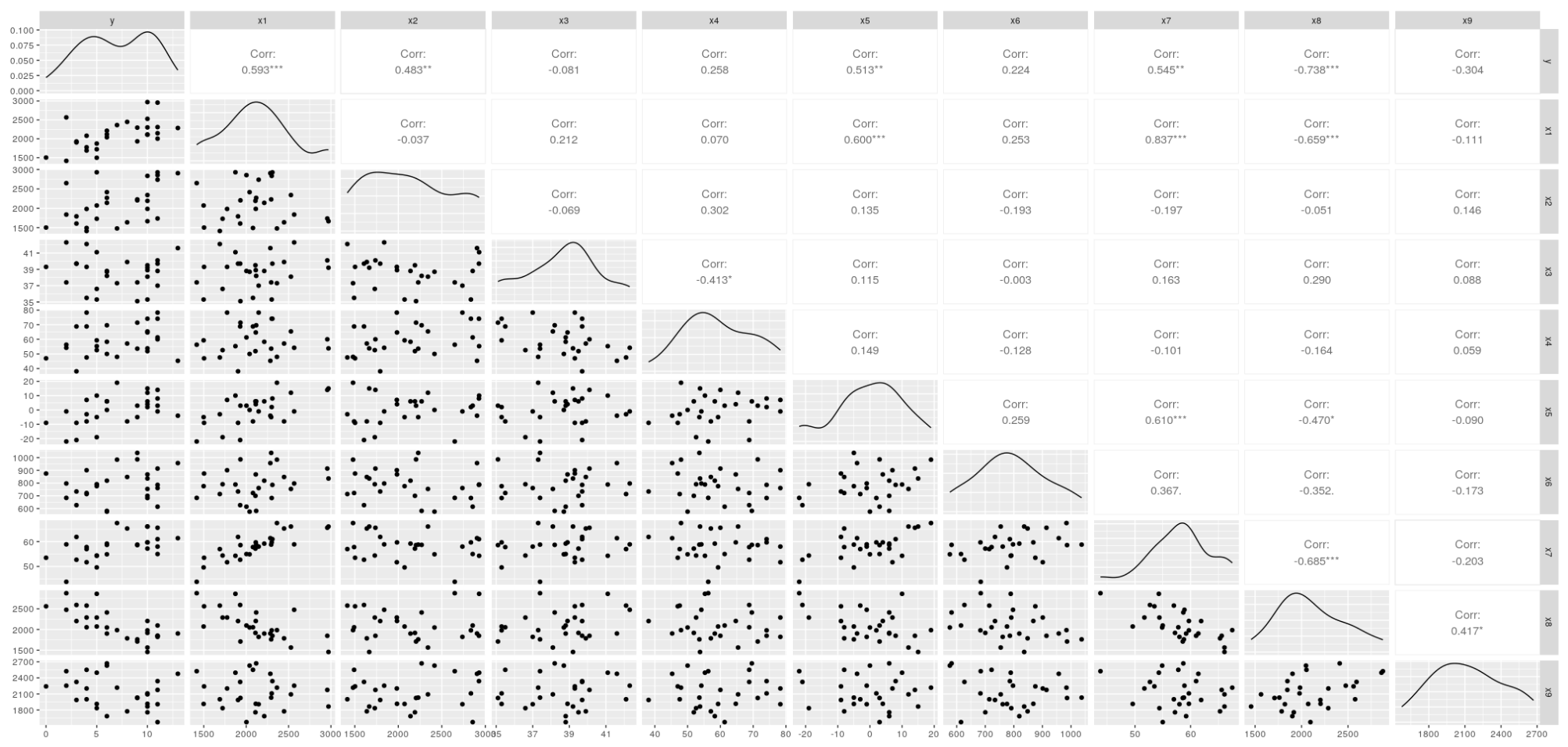
We can see that a few variables stand out in their correlation to Games won; Rushing yards, passing yards, Opponents’ rushing yards and Opponents’ passing yards have the highest correlation coefficients. But this doesn’t tell us everything we’d like to know about what makes a good model. Specifically, a model using these variables definitely seems to run the risk of multicollinearity, and our coefficients may become distorted. Apart from that, would a mixture of other variables make an improvement? Would Rushing yards and Field Goal Percentage make a better model than just Rushing yards? A conventional approach to this problem may be to use some criterion for variable selection. The below shows code output from using the ols_step_both_aic() method for variable selection from the olsrr [3] library.
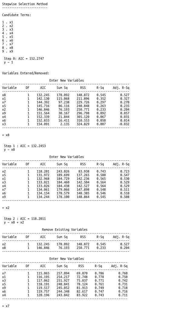
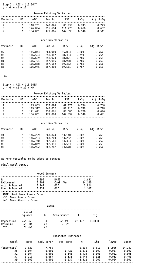
So according to this variable selection method, the final model output yielding the lowest AIC score is: y ~ x2 + x7 + x8 + x9. We can see that the previously observed high-correlation variables are included. But we are left with a few problems. For instance, why wouldn’t Rushing yards, the variable with the highest correlation to Games won be included? Is it sufficient to say that the other variables can do the work of explaining the effect of Rushing yards? How would we reason about that in real terms? Another problem we have is the y-intercept given by the final model. Given no information about a team, this model tells us we should expect -1.88 games won (with a standard error of 7.785). How can we expect a negative number of games won? And doesn’t this relatively huge standard error lower our confidence?
One of the issues with relying on an unexamined strategy for variable selection is that it doesn’t promise to make the model interpretable. That is why we don’t have answers to the questions above. An overarching mistake is that the approach overlooks the zero-sum game dynamics in football. More rushing and passing yards might not reliably predict more games won if it coincides with a relatively higher number of yards made by opposing teams. Likewise, a low number of offensive yards could be associated with a high number of wins, if that team happened to keep their opponents yardage sufficiently low. Shorter punts, more turnovers, and more penalties may not matter in the end if offensive yardage is kept low.
So is there a way to incorporate this knowledge into the model? There is. We can create a new variable that simply takes the difference between a team and their opponents total yards:
differentialYards <- (x1 + x2) - (x8 + x9)
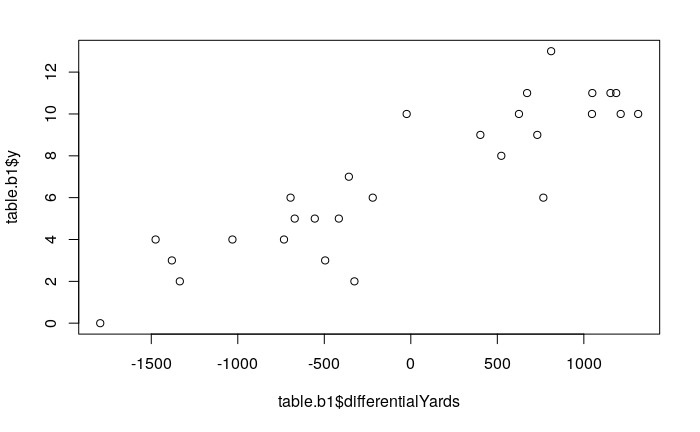
Differential Yards tells us how much more or less yards a team gained relative to their opponents. This variable now captures inherently some of the two player min-max game dynamics. A scatter plot shows it has a stronger and sharper linear relationship with Games won than its component variables do individually. As an experiment, we can run variable selection again to see how it compares to the other variables:
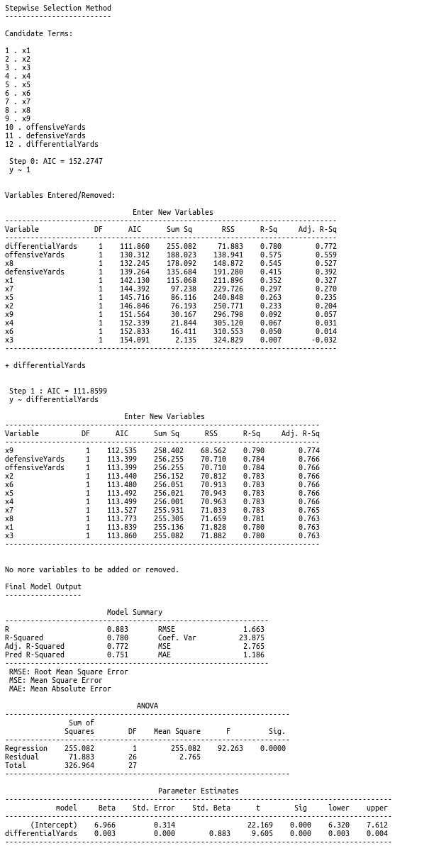
In this run, Differential Yards is the only variable that meets the selection criteria. Not only that, we have a very interpretable set of coefficients. The y-intercept is approximately 7, meaning that without any information about a team this model predicts that it will win about half of its games. This is a reasonable expectation. Likewise, every Differential yard made by a team contributes to about 0.003 more games won. Given that the field is 100 yards, this is definitely on the proper scale for reasoning that 100 more differential yards means roughly another touchdown, which may be somewhere near adding 0.3 more wins in a season, which is reasonable as the average number of touchdowns in NFL games is somewehere around 3 or so. We also don’t have to rationalize anything about the way a yard is scored. What does it matter that a team made a yard via a pass or a rush? In terms of winning, it only matters that they gained a yard.
Giving some thought to the events themselves that are being model can go a long way in improving model performance and interpretability. It is often the case that this kind of thinking can’t be done by some predetermined set of statistical tests, but requires the ability to make abstractions.